Time Evolution - Line Chart

Create a line chart

Suppose we are interested in following the evolution of weekly hospitalisations in Switzerland over the last 2 years, and would like to create a new chart for that, using the switzerland.foph_hosp_d dataset.

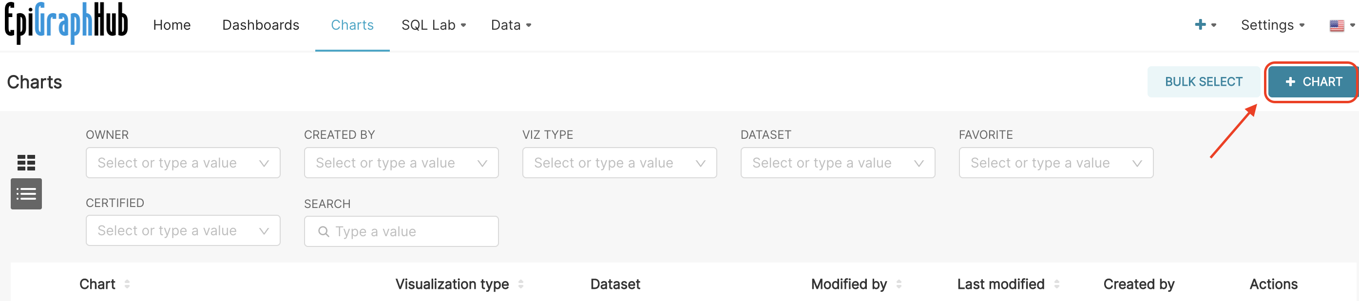
Let’s go back to the Charts page, and click on the +CHART button in the upper right corner of the page to create a new chart.

{width=”750px”}

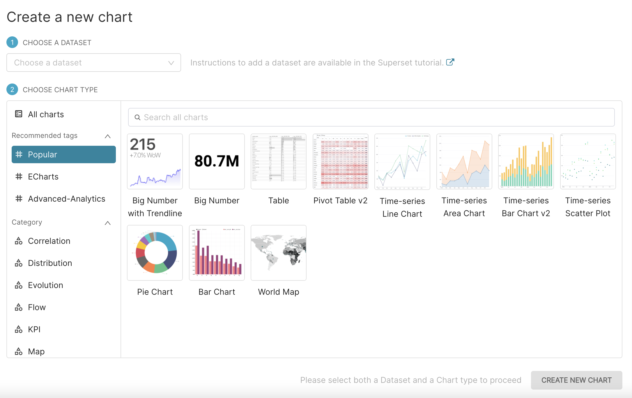
The page named Create a new chart opens. You must do two things here:

1. CHOOSE A DATASET, and

2. CHOOSE A CHART TYPE.

{width=”750px”}

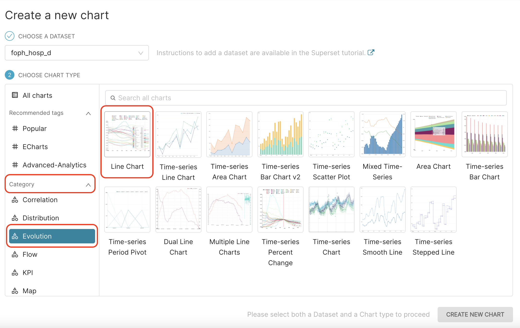
In the field CHOOSE A DATASET, type or select from the drop-down list again the foph_hosp_d dataset.

In the CHOOSE CHART section, different sub-sections are available: Recommended tags, Category, and Tags.

In the Category sub-section, select the Evolution category. A number of corresponding charts will appear on the right panel. Let’s click on the first one and select the: Line Chart. It is the classic chart that visualised how metrics change over time.

{width=”750px”}

We can then click on CREATE NEW CHART button in the bottom.

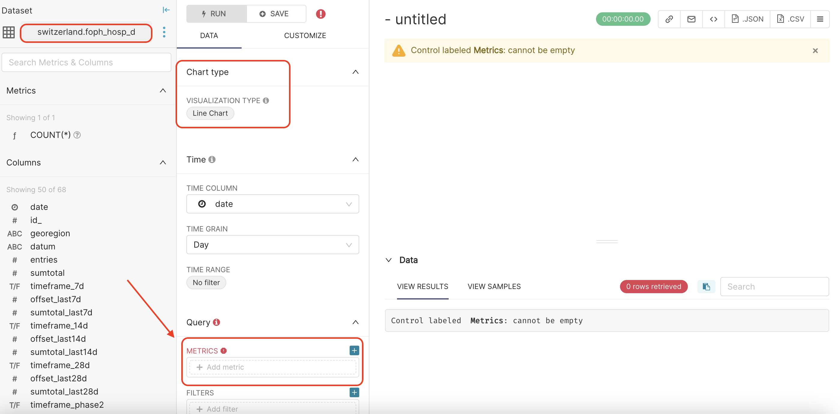
When you do so, a new Chart page opens, with pre-filled Dataset and Chart type fields.

You can see as well that for this type of chart, some parameters are mandatory. It is the case here for the METRICS field in the Query section. That is why it is colored in red, and annotated with an exclamation mark (!). Indeed, for line charts, METRICS field cannot be empty and one or many several metrics must be selected to be displayed.

{width=”750px”}

Metrics and Aggregation

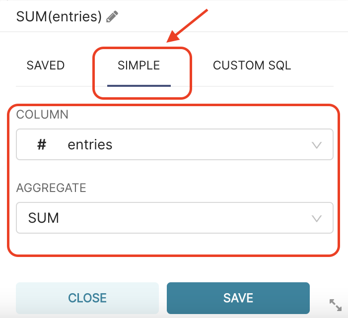
As at least one METRIC is mandatory, let’s click on + Add metric in the METRICS field. A pop-up window appears. When we select the SIMPLE menu, we are requested to fill the COLUMN to be displayed and how we would like to AGGREGATE it.

As we have daily new hospitalisations data in our dataset and we are interested visualising weekly hospitalisations, we will set COLUMN to entries, and AGGREGATE to SUM, since the number of hospitalisations (entries) per week is the SUM of the daily hospitalisation during that week :)

{width=”250px”}

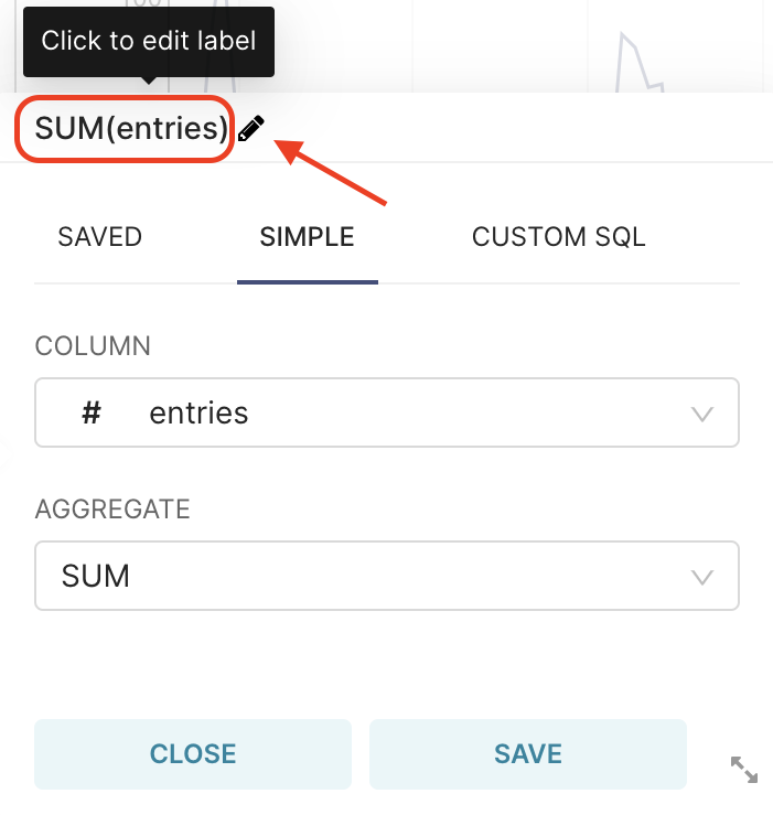
::: side-note Based on your definition, this metric is now labeled SUM(entries). Unless you edit it, this is the label that will appear in the legend of your chart.

To edit the label of this metric (e.g. change it to “Number of entries”), click on the pencil icon, highlighted below:

{width=”250px”}

:::

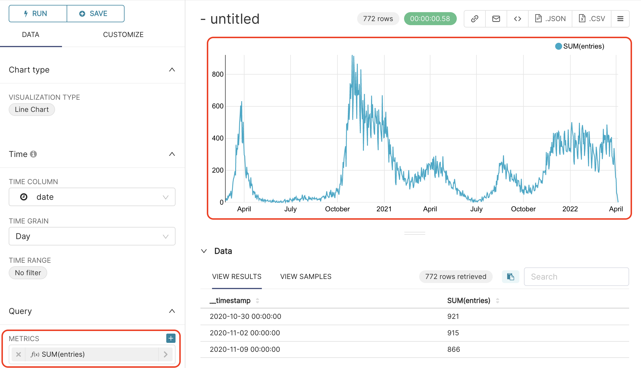
When you are done, click SAVE in this pop-up window, then click RUN QUERYon the right panel of the Chart page. The result should be the following:

{width=”500px”}

Time grain

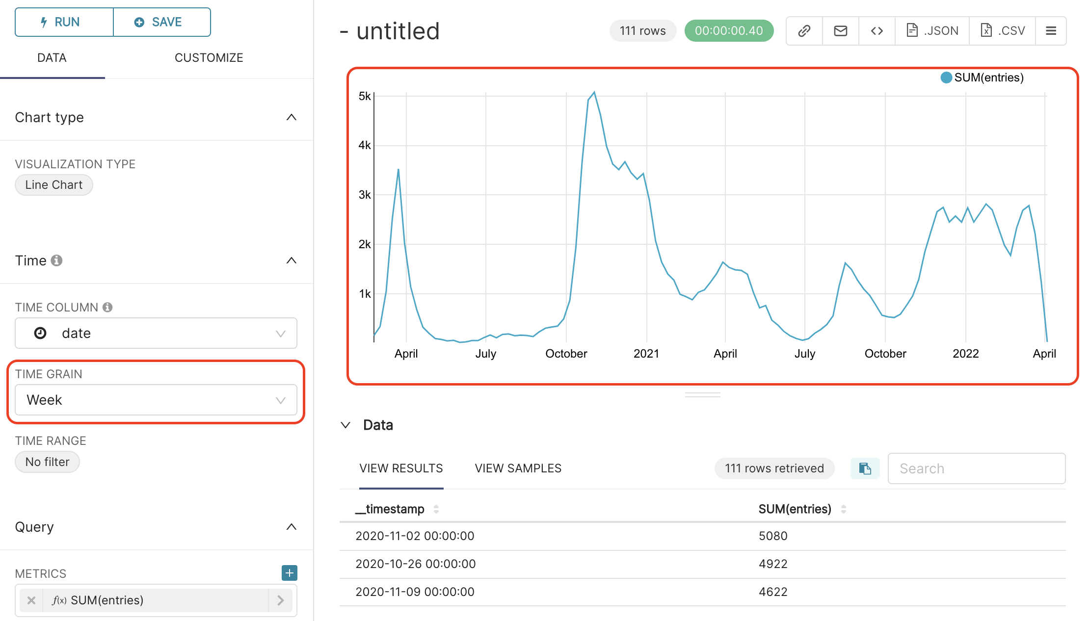
By default the TIME GRAIN field in the Time section is set to Day. As we are interested by numbers of weekly hospitalisations, let’s change it to Week, for aggregating entries at the weekly-level, and RUN QUERYagain. You will get the result below, where you can directly see how it made the line smoother.

{width=”500px”}

Group by Swiss Canton (State)

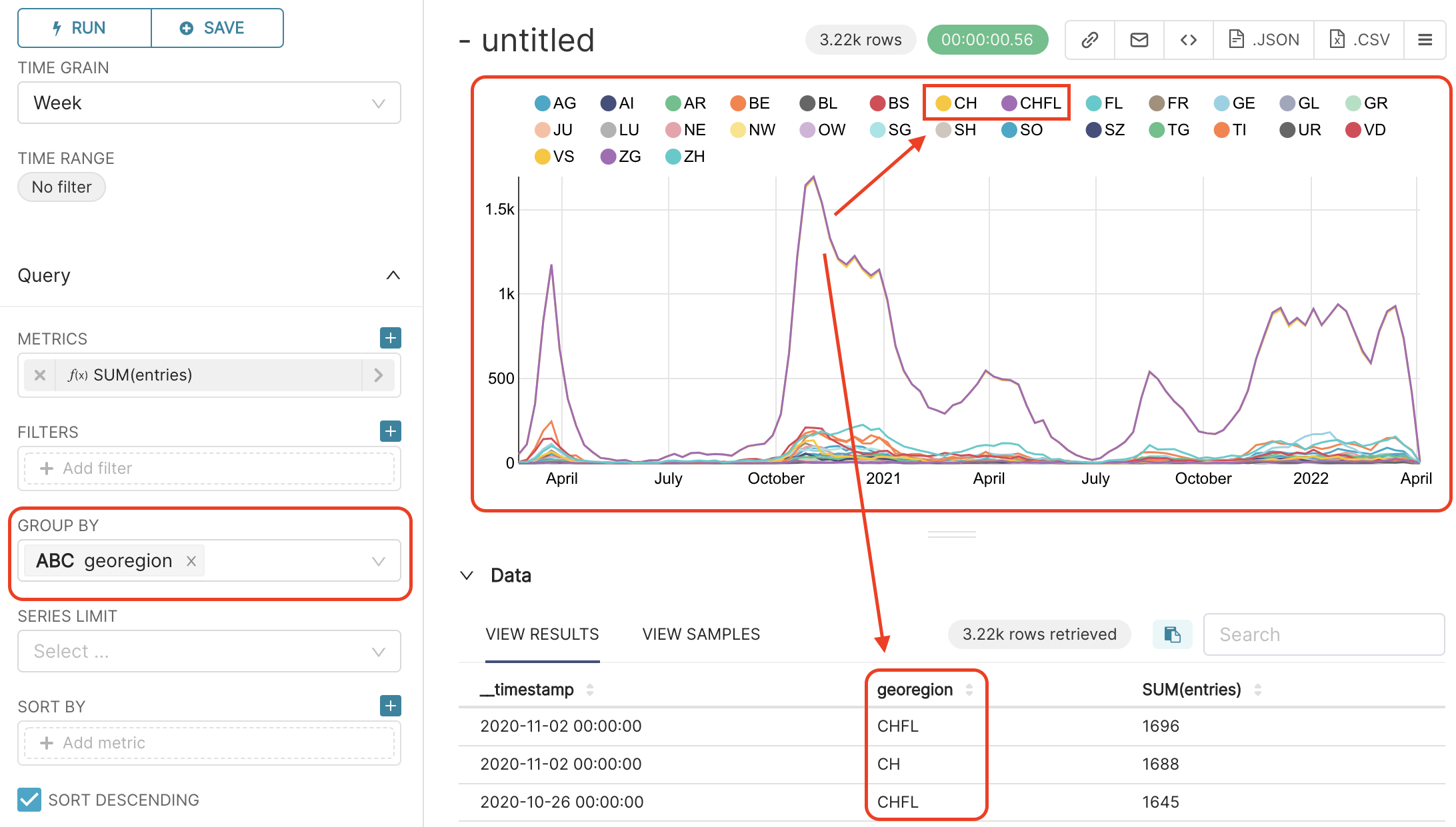
Currently all entries in our table (independently from georegion value) are summed by week. Let’s GROUP entries BY georegion, to see the evolution of the number of entries by georegion (Swiss canton).

In GROUP BY field, add georegion column, and press on RUN QUERY.

The results should look like the following:

{width=”500px”}

Great! We can see now that data are separated by canton. But, we also see that we have data for the whole Switzerland (georegion = CH) and for Switzerland and Liechtenstein (georegion = CHFL) all together.

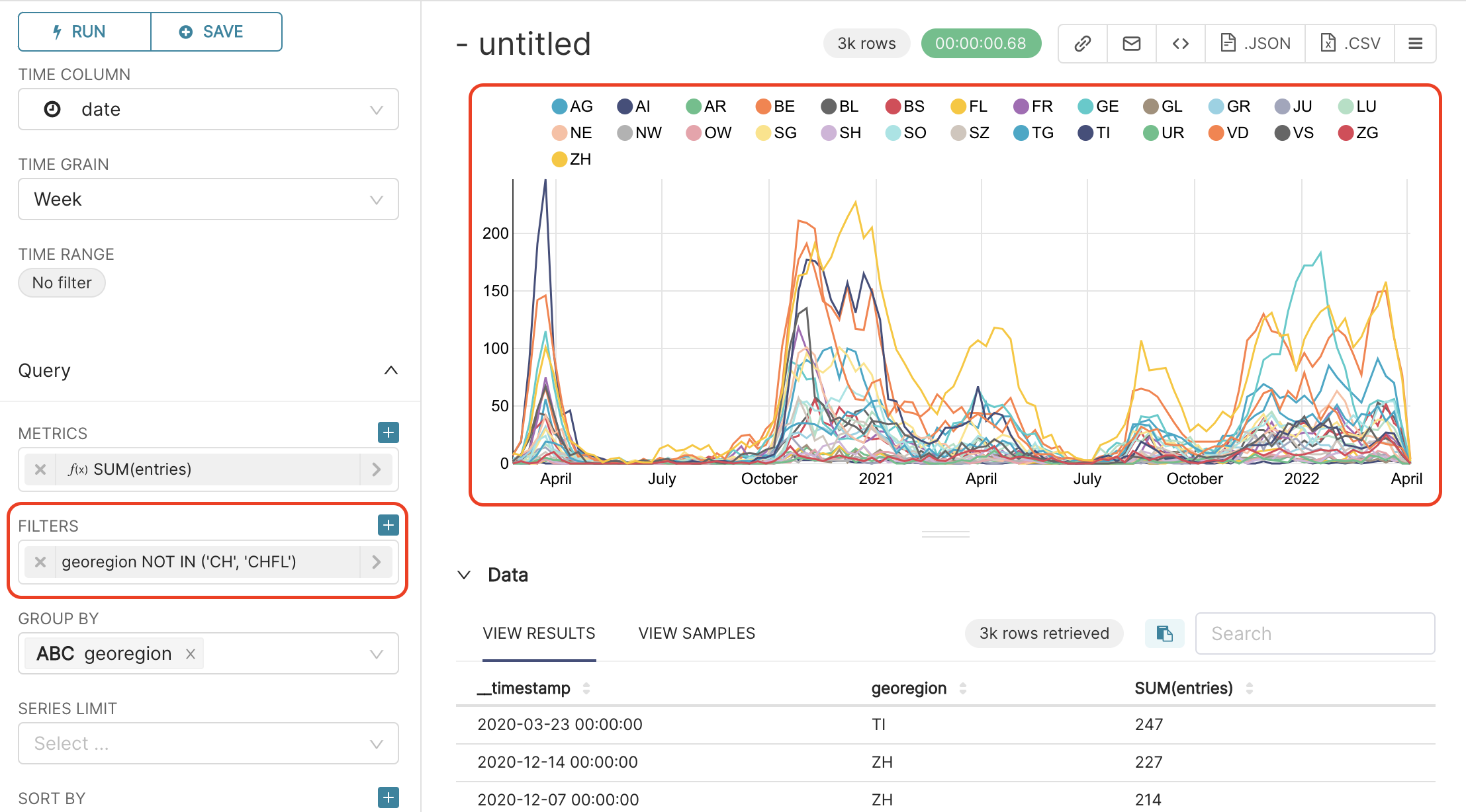
Filters

In order to focus on canton data only, we must FILTER out CH and CHFL data. In FILTERS, click on +Add filter, and set the filter to georegion NOT IN (CH, CHFL).

{width=”500px”}

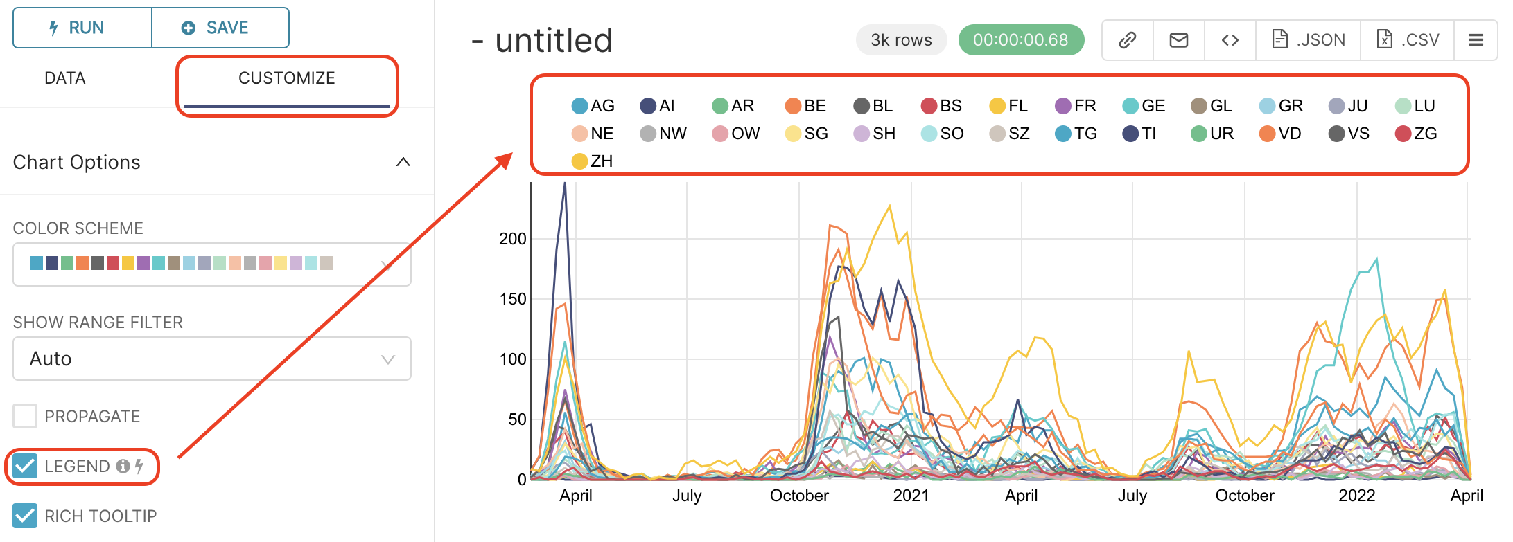
Finalise chart: Legend, Axes, Title

• In case a legend was not added automatically, when you grouped by georegion, add it to see the correspondence between the line colors and the cantons. For that, go to the CUSTOMIZE tab (next to DATA tab), and tick the LEGEND box.

{width=”500px”}

Note that the plot is interactive; you can show or hide lines from the chart by clicking or double-clicking on their associated legend item!

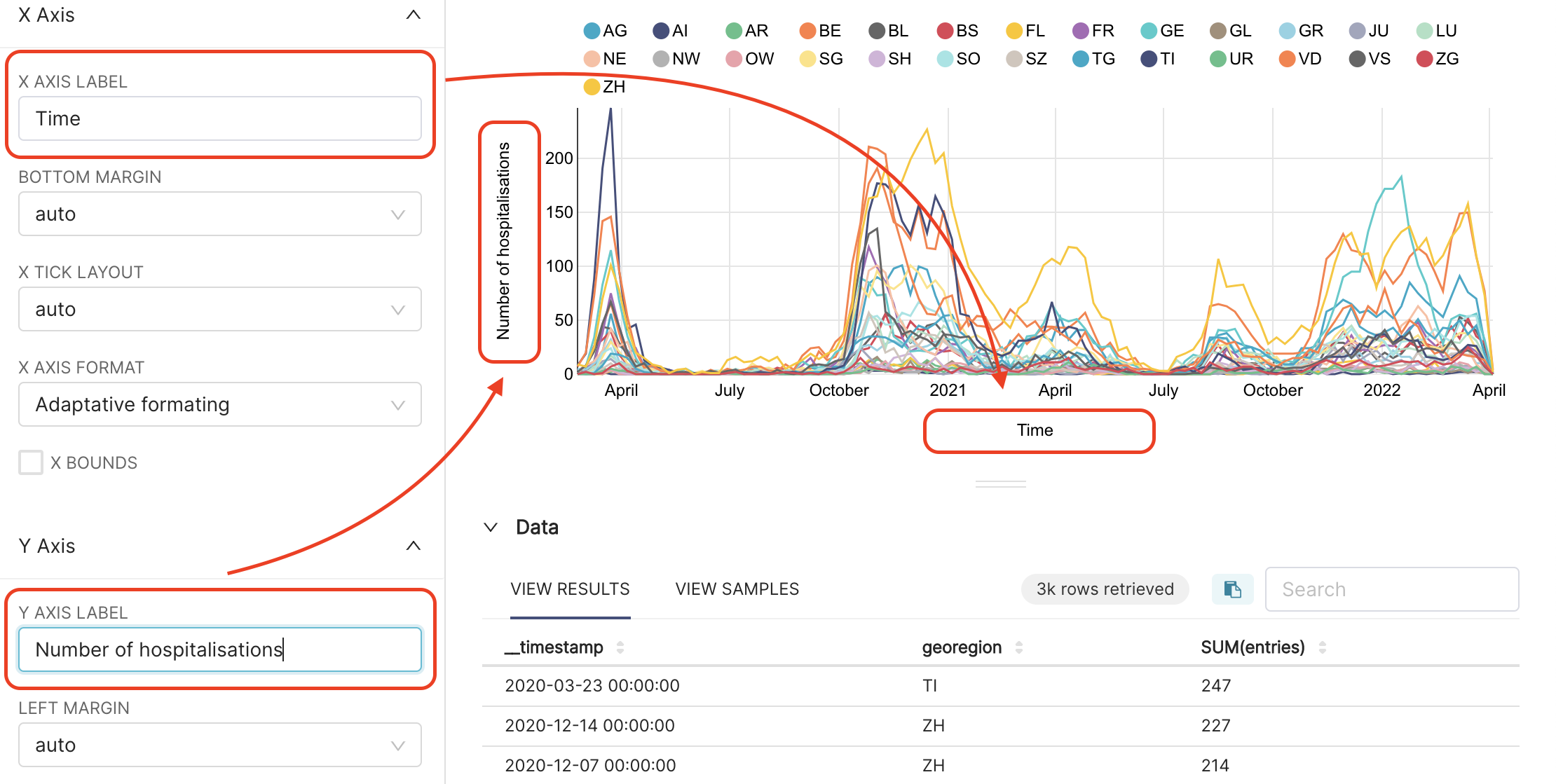
• While we are in the CUSTOMIZE tab, let’s also add a name to the X and Y axes. In the X Axis section, write Time in the X AXIS LABEL field, and Number of hospitalisations in the Y AXIS LABEL field of the Y AXIS section.

And that’s the result, where we can see the different waves during the last 2 years, by Swiss canton.

{width=”500px”}

Finally, let’s give a title to this line chart, for example Evolution of weekly COVID hospitalisations in Switzerland by Canton.You can save it, by clicking on +SAVE button in the middle panel.